B June 2017 clipping volume report
I prepared this progress report in June 2017 to share information with turf managers who shared clipping volume data with me over the past few years.34
Introduction
I now have data on clipping volume from putting greens on nine golf courses. For many of these courses there are data from multiple (or all) greens at each mowing; for some of the courses there are data for a selection of indicator greens, or for a single green. This report gives a summary of the data collected so far, with some advice on how the data can be understood and used, and with an explanation of what I’m trying to learn from these data.
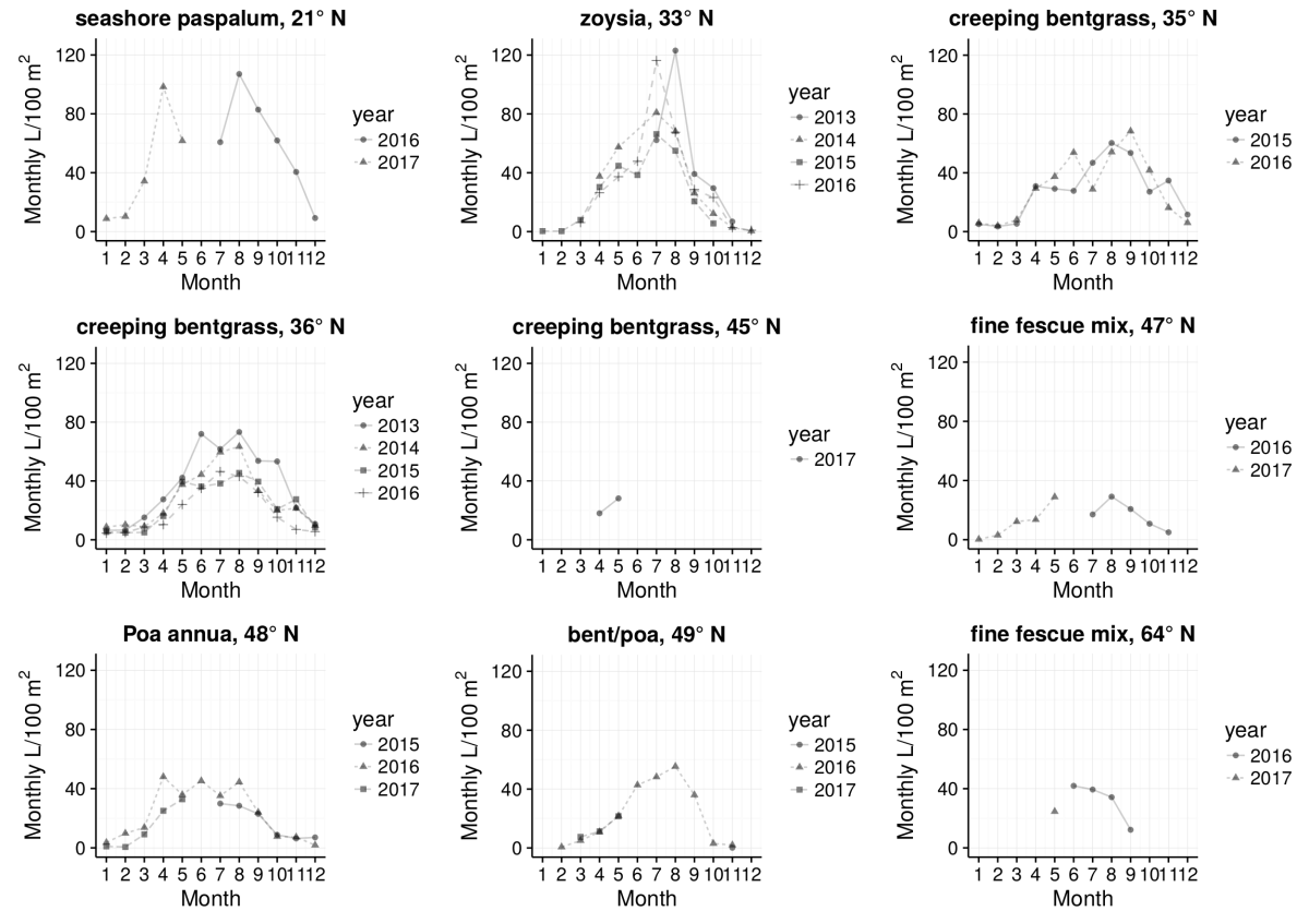
Clipping volume data from 9 locations as of May 2017
The previous page shows monthly totals for the nine locations.
B.1 What’s the use of clipping volume?
In Short Grammar of Greenkeeping I wrote that a way to define greenkeeping is to say it is “managing the growth rate of the grass to create the desired playing surface for golf.” The typical way to assess growth rate is to observe the grass, and also to observe the quantity of clippings. Because clippings from putting greens are collected in mower baskets, it is a simple procedure to measure the volume of clippings as the mower baskets are emptied.
I can think of many ways that these data might be useful, but the volume data need to be put into context, or have some baseline comparisons, before one can be confident in changing maintenance practices based on them. Here’s what I’m usually thinking of when I consider clipping volume data:
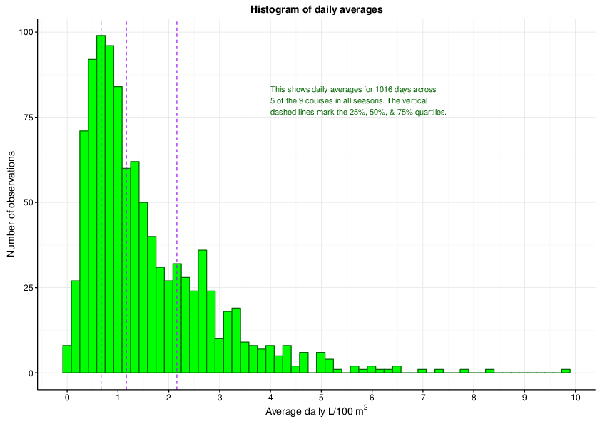
The median value for clipping volume is 1.2 L 100 m-2 and 50% of the measurements are from 0.67 to 2.2
- growth rate tracking
One might have a target growth rate for certain seasons, for cumulative amounts to match traffic, or target rates for special events. Big tournaments might have lower growth rates. Busy seasons of golfing traffic might require faster growth rates. One can compare from course to course, or one can compare within the same course from year to year or season to season. I have been using units of liters (L) of clippings per 100 m2 of green area. There is plenty of variation, and that is normal. To pick the center of the variation, I can describe the median values. When putting greens are mown, the growth rate is such that 50% of the time the volume is from 0.67 to 2.2, with a median of 1.2. That’s for all seasons and doesn’t correct for number of days since the last mowing. That’s just what is in the baskets, and the histogram in Figure 1 shows what to expect. If you are getting less than 0.67, then that is in the lower 25%. That’s not much growth. And you might sometimes get from 2.2 up to about 10, but that is rather high. This is not to say what any course should be, but is an attempt to put this into context.
- checking consistency or variability
Are all greens growing at the same rate? Are all the mowers cutting the same amount of grass? Is anything changing across the course as a whole, or on a subset of greens? Having a number for the amount of leaves being cut off the greens helps to answer those questions.
- adjusting inputs based on growth
It seems reasonable in the day to day operations of a golf course to consider making adjustments in the N supply, mowing height, topdressing rate, growth regulators, rolling frequency, irrigation rate, etc., based on how much the grass is growing and how much the actual growth rate deviates from the desired growth rate.
- estimating the real growth
Volume is measured because it is easy. What can be even more useful is the dry weight of the clippings harvested, but that is not practical, for two reasons. First, one needs to separate any sand collected in the clippings from the clippings themselves. Second, one must dry the clippings in an oven. But one can make an estimate of the dry weight from the clipping volume.
- estimating nutrient use and harvest
Now we move on to topics that are of particular interest to me, perhaps more from a research perspective rather than turfgrass management. But if we have an estimate of the dry weight harvest, then we can estimate nutrient removal through mowing on a daily, weekly, monthly, and annual basis. If we know nutrient use, then we should be able to match that with nutrient supply. We can also compare locations. For example, if location X used this much N and K and had a known growth rate, then location Y turf management can be adjusted based on how location X was managed.
- topdressing and organic matter management
Wouldn’t it be nice to never topdress? To never core aerify? If the surface conditions were perfect, and then the growth rate was 0, one would never have to topdress or aerify. I am interested not so much in eliminating topdressing or aerifying, but in trying to understand how this work can be done as little, or as infrequently, as possible. It seems likely that knowing the growth rate, and then comparing what is done at location X and Y, one can get closer to the objective of doing that work as infrequently as possible.
- checking temperature and growth potential
When I first started looking into this, it was largely on this topic. I was less interested in the actual amount of growth, and was more interested in how it was related to temperature or temperature-based growth potential. See, for example, this report from 2014: http://www.seminar.asianturfgrass.com/20140612_clipping_yield.html. I’m less interested in that now – more about that later.
In some of these areas, I have a pretty good idea of what the numbers mean. In others, I don’t, but I want to learn more and see if it is possible to make use of the clipping volume data to get to an answer. Here’s a summary of where I’m at so far.
B.2 Growth rate tracking
I really started to get interested in these clipping volume data while working with Andrew McDaniel at Keya GC during the KBC Augusta tournament. I’ve written about this here: http://www.blog.asianturfgrass.com/2015/09/tournament-week-clipping-volume.html. To produce the desired putting surfaces for the tournament, it was really helpful to check the clipping volume data. As I looked into this more, I saw how easy it was to collect the data, and I realized that there were a lot of uses for these data.
The second page of this report shows total amounts by month for different grasses at different locations. From a look at that, you can see what the normal amounts of clippings tend to be. Figure 1 shows the clippings you can expect on a single day. But of course that is bound to vary by season. I think it makes sense to be familiar with the normal ranges and fluctuations at your course, and also to know what is normal in the big picture of all courses.
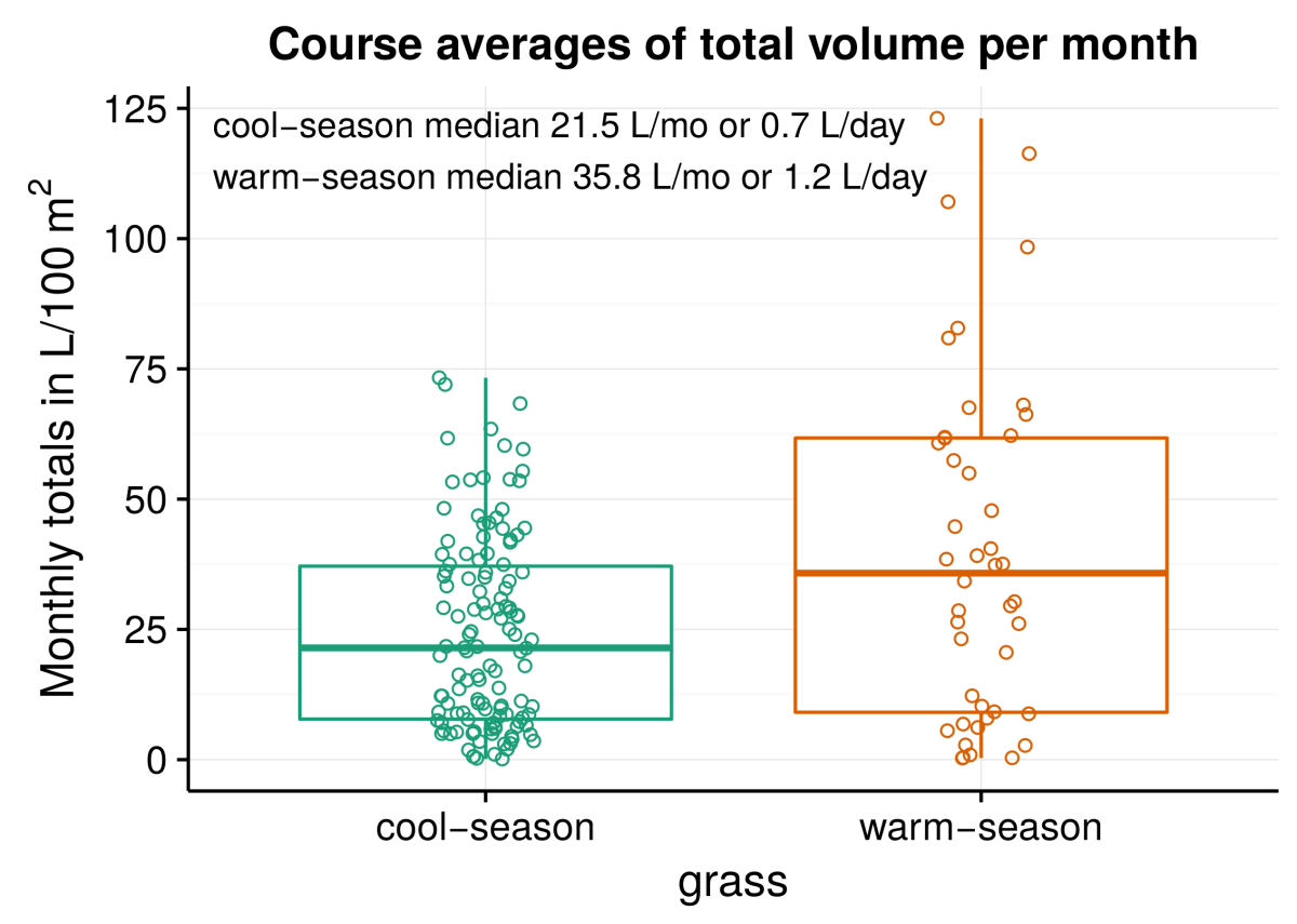
This boxplot shows the monthly totals for all nine courses. If one divides the total volume in a month by the number of days in the month, the result is an estimate of how much the grass is growing on a per day basis.
Figure 2 shows the cool-season and warm-season monthly totals. Remember, this is for all months, so it includes some months when the grass is only mown a few times. But it generally represents what is typical over a long period of time.
B.3 Checking consistency or variability
This is something I am really interested in. I know some places just test one green, and use that to track some data. I find in most interesting when all the greens are measured, because one can then check that all mowers are cutting the same, and can evaluate the microenvironments on the course that may influence growth, and can check the consistency of the measurements.
I’ve spent a lot of time working on this, and don’t have a perfect answer yet. If you are really interested in this, please have a look at http://www.blog.asianturfgrass.com/2016/08/clipping-volume-variation-from-green-to-green.html and especially check the charts I showed in that post.
The best I can come up with now is this. When measuring all the greens (or multiple greens), the median coeifficient of variation (CV) is about 0.33. The coefficient of variation is the standard deviation of all the measurements, divided by the mean (average) of all the measurements. That would be for a single day. If the CV is less than 0.33, you can think of the greens as being more consistent than normal. If the CV is more than 0.33, and as it moves above 0.4, then you can think the clipping volume is less consistent than normal. The CV is not exactly like going up or down by a fixed percentage, but I think it is reasonable to look at it this way. If you measure say 18 greens, or 20 greens, or even 3 greens, and want to check the consistency, but don’t have an easy way to calculate the CV, just take the average (mean) and then go down 33% and up 33%. If all the clipping volumes are within those boundaries, then the greens are more consistent than usual. If one or more greens are outside those boundaries, then the greens are less consistent than normal.
I’m still working on this, so if you have suggestions, I’ll be happy to hear them. I prefer the coefficient of variation to describe the variability in multiple numbers. I looked up the standard equation for defining what is an outlier, and that is 1.5 times the distance from the 25% quartile to the 75% quartile. 50% of the measurements will be in that range, and one can take that range, multiply by 1.5, and then add to the mean, and subtract from the mean, and then check if any measurements are outside that range.
I prefer the CV to this outlier identification approach because I think it more accurately represents what we would be looking at. Here’s a quick example with green speed to illustrate this.
Let’s say we measure five greens with a stimpmeter. The greens have a speed of 9, 9, 10, 11, and 11 feet. The average (mean) is 10 feet. The standard deviation of those greens is 1 foot. That is, the average green is 1 foot from the mean. The CV is then 0.1.
We could also have five greens with a speed of 9, 9.5, 10, 10.5, and 11 feet. Now the standard deviation goes down, because two of greens move closer to the mean which remains at 10. The standard devation of those five greens is 0.79 feet, and the CV is lower than 0.1; it is now 0.079. The CV tells us something here. It shows which set of data have less variation from the average value.
If we would take the outlier identification approach, it doesn’t identify any outliers.
B.4 Ajusting inputs based on growth
I don’t have any numbers to share here, but if I were managing turf, I’d be adjusting inputs based on how much the grass was growing. I’d look at the grass, and I’d look at the color of the grass, and I’d check the weather forecast, and I’d consider the current grass conditions and how those compare to what I want the future grass conditions to be. To those data or observations, I’d add the clipping volume data, and take these all together to make better choices about what to do and what to change. How to adjust the dials of the inputs to get the desired turfgrass conditions, as Chris Tritabaugh has explained to me.
B.5 Estimating the real growth
Volume is kind of useless. What we really want is dry matter harvest. That is how much the grass grew, not counting water. How much actual plant material was produced, per surface area of turf? While volume is useless, it is easy, and from volume we can estimate the dry matter yield.
B.6 Fresh weight of clippings
I think volume is the easiest thing to measure. To measure fresh weight one must bring along a scale, or bring the clippings back to a scale. And then there is the issue of the water in the clippings, and the sand in the clippings. Sand is going to affect the volume too, but I think sand will have proportionately more effect on the mass of the clippings.
Andrew McDaniel35 has shared 2016 data with me of volume and fresh weight measured from the same greens (Figure 3).
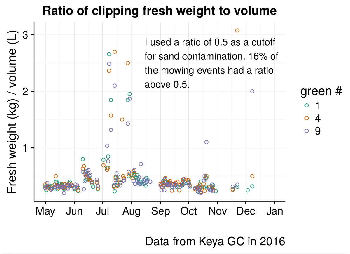
The ratio of fresh weight to clipping volume for grass clippings collected from three greens at Keya GC in 2016.
This is for korai greens, and the ratio may be different for other species. But for korai, as Figure 3 shows, when the ratio of mass to volume is more than 0.5, that is when there is a lot of sand on the greens. These data are being collected again in 2017 at Keya. In 2016, 16% of the mowing events had so much sand in the clippings that the data had to be discarded, if we use that 0.5 ratio cutoff rule.
But after getting rid of the samples that are contaminated with sand, there is a consistent relationship between fresh weight and volume (Figure 4). To reiterate, I prefer to measure clipping volume because volume is easier to measure, and because volume has less of a problem with sand mass error. And after one has measured volume, one can predict the mass anyway.
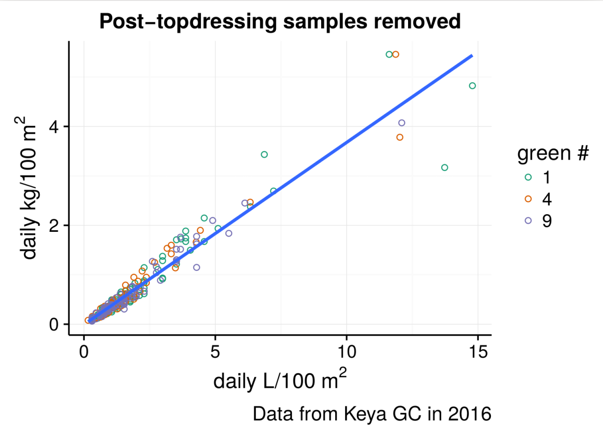
The clipping volume has a consistent relationship to the fresh weight of the clippings when sand-contaminated samples are removed.
B.7 Estimating nutrient use and harvest
This is something I find really interesting. If we can estimate the dry matter harvest from the clipping volume, then we can have an idea of how many nutrients the grass is using. Mr. Kihara and Mr. Seiyama from Nichino Ryokka carefully collected clippings and measured volume, fresh weight, and dry weight at the Nichino Ryokka research center in Chiba. Figure 5 shows the relationship between clipping volume and clipping dry weight (there is a drying oven at the research center) for three different grasses.
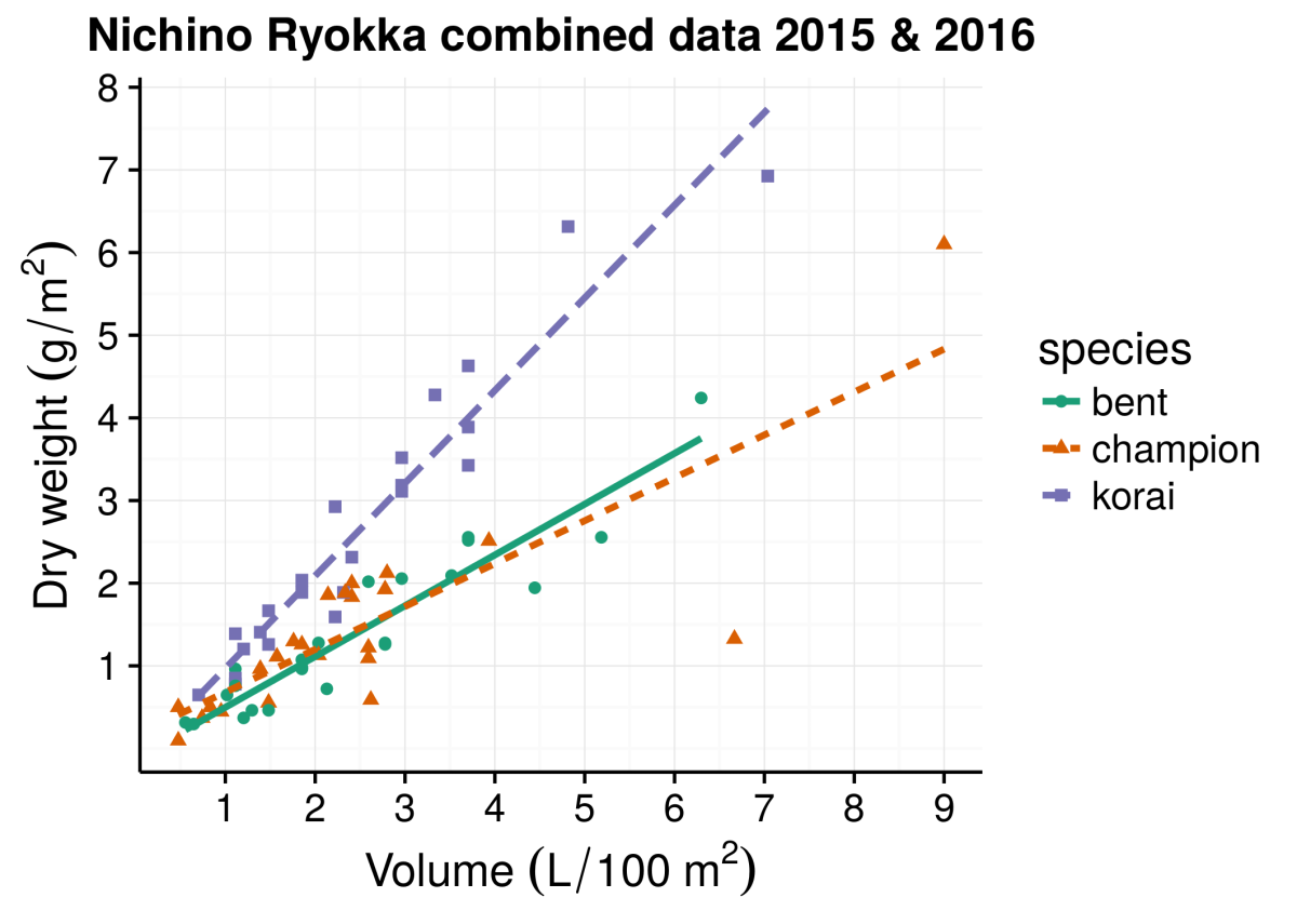
Data from the Nichino Ryokka research center show that dry weight of grass clippings can be predicted based on the clipping volume
If we focus on creeping bentgrass and Zoysia matrella (korai), I’ll quickly explain how this works. First, let’s do bentgrass. The slope of the line (in Figure 5) for the bentgrass volume to dry weight relationship is 0.63 g m-2 for every 1 L 100 m-2. The bentgrass greens at the location 36 degrees North latitude have an average annual yield in volume of 326 L 100 m-2. That works out to an expected annual clipping harvest of 205 g m-2. If the bentgrass leaves have 4% N, that is 8.2 g N m-2. The N applied to those greens in 2014 was 12.9 g, then 10.1 in 2015, and I don’t have the final numbers for 2016 but it was less than 10. So there seems to be a pretty close correspondence between the N applied and the growth.
For korai, I’ll use the data from the zoysia at 33 degrees North. The average clipping volume from 2013 to 2016 at this location was 340 L 100 m-2. From the Nichino Ryokka data, we can expect each liter of korai clippings in 100 m2 to work out to 1.1 g of dried clippings in 1 m2. That gives an expected harvest of 374 g m-2, and if the korai clippings have 3% N, that would be a N harvest in the clippings of 11.2 g m-2. At this location, the N applied from 2013 to 2016 was 14.6, 9.5, 10.6, and 11.1 g m-2. We can work through this for every element. I just show for N to point out that in the case of profesionally-managed turf (both the bentgrass and korai course used as examples here host professional tournaments too) supplied with a relatively low amount of N fertilizer, the quantity of clippings produced is related to the quantity of N supplied.
The implications of this are that one can be more precise in nutrient applications. And I am interested in this as a way to check nutrient depletion rates from the soil, and do some calculations related to the MLSN guidelines. I think for most turfgrass managers, it is enough to understand that the clipping harvest represents a quantity of nutrients, and also the fertilizer applied represents a quantity of nutrients. This particular aspect is more of a research thing, rather than a turf management thing, but I am especially interested in this.
You can imagine what I think of supplying two or three or more times the quantity of an element, like potassium or phosphorus or calcium, compared to the amount that is used by the grass. These calculation are a way to document this.
B.8 Topdressing and organic matter management
But this growth, as it relates to the nitrogen supply, is quite pertinent to this section. I don’t have too much to say here, other than it makes sense to me that if the grass grows less, by less N supply, then there will be less of a need for topdressing and core aeration.
If you haven’t, see http://www.blog.asianturfgrass.com/2016/05/data-to-support-an-anecdote.html for more about this. This is about a course doing 45,000 rounds per year and that has dormant grass for 6 months. The N supply is low, the grass conditions have gotten better year after year, and the soil organic matter keeps going down. But the core aeration and topdressing are also less than what you might expect.
I believe this approach can be implemented in more places. And I think measuring clipping volume can be a way to compare locations. So if X location is having great success with this much topdressing and this much N and this much clipping volume, I think the clipping volume comparison from place to place can be used to fine tune some of the organic matter management. I’ve written articles about this in my series for Golf Course Seminar magazine, in particular I think the March and April 2017 issues. When I get the 2nd edition of Short Grammar of Greenkeeping to the printer, those articles (in English) will be included as appendices.
B.9 Checking temperature and growth potential
This was my original interest in this, and I am still working to understand this. There is obviously a relationship – look for example at seashore paspalum at 21 degrees North – it grows less in winter. Look at fine fescue mix at 64 degrees North – it doesn’t grow in winter. At the broad scale, temperature plays a huge role. Actually, looking at all the charts again, it is easy to see how much of a seasonal – a temperature – effect is there.
As I’ve become interested in predicting dry weight of clippings and nutrient use of grass, and also trying to understand what normal variability of growth is, I put the temperature analysis on the back burner. I’m still really interested in this, but there is only so much time to work on it!